From python API
Analyze Dataset
Tha analysis is based on:
- Silhouette index: The silhouette value is a measure of how similar an object is to its own cluster (cohesion) compared to other clusters (separation). Therefore, as high as possible the better.
- Calinski-Harabasz index: The score is defined as ratio between the within-cluster dispersion and the between-cluster dispersion.
- David-Bouldin index: The score refers to a model with better separation between the clusters.
from sklearn import cluster, datasets, mixture
import cluster_drug_discovery.methods.kmeans as ks

X, y = datasets.make_blobs(n_samples=1500, random_state=170)
cluster = ks.KmeansAlg(X, nclust=3)
cluster.analyze()
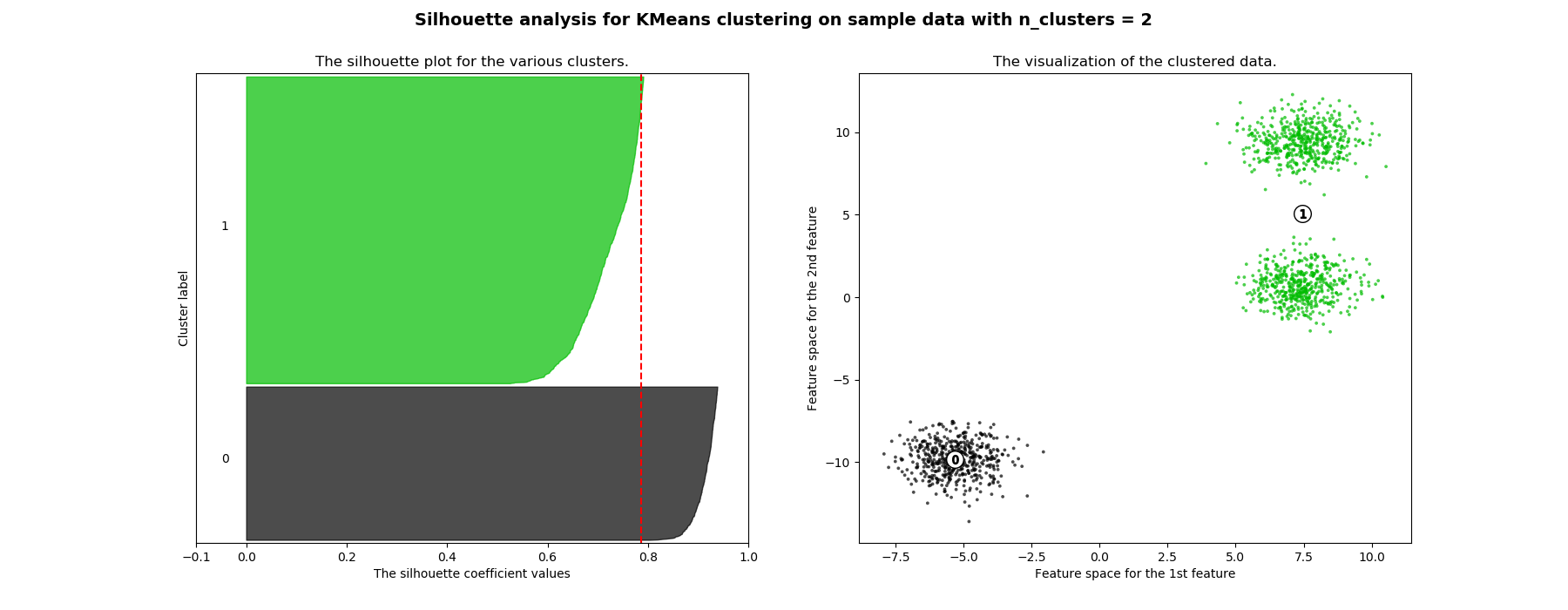
Silhouette
As seen in the pictures belowe as high the silhoutte coeficient is the better the clustering. As the silhoutte coefficient give us a sense of how separate each point is from the other clusters.
Therefore, when we move from 3 to 4 clusters the silhouette index of the first and second cluster clearly drops as they are next to each other in the feature space while with nclusters=3 all clusters were very separated.
In case of having a 2D dataset the plot will be the values of the samples. If the dataset is 3D or higher the plot will show the first two pca components. However, we will retrieve umap plots to include non linear dimensionallity reduction techniques. (Learn more three sections below)


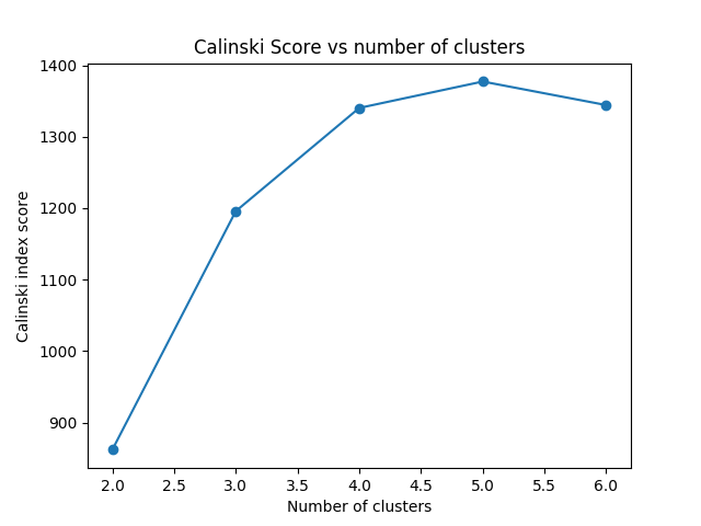
Carlinski
In terms of the Calinski-Harabasz index the score is higher when clusters are dense and well separated, which relates to a standard concept of a cluster. The score is fast to compute. Whereas, The Calinski-Harabasz index is generally higher for convex clusters than other concepts of clusters, such as density based clusters like those obtained through DBSCAN.
As seen in the plot belowe as Calinski index is based only on density it gives a better score for ncluster=4 than ncluster=3 as the clusters are smaller and therefore more dense. However, that does not mean that the result is better. In conclusion, this index give us usufull information about the cluster density but must be use with other indexes like the silhoutte.
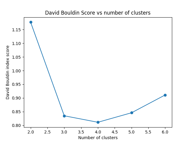
David-Bouldin
The David-Bouldin score refers to a model with better separation between the clusters since algorithms that produce clusters with low intra-cluster distances (high intra-cluster similarity) and high inter-cluster distances (low inter-cluster similarity) will have a low Davies–Bouldin index, the clustering algorithm that produces a collection of clusters with the smallest Davies–Bouldin index is considered the best algorithm based on this criterion.
As seen in the plot below we can clearly differenciate that moving from nclust=2 to nclust=3 the intra-cluster distance gets better. However, from nclust=3 and nclust=4 the intra-cluster distance remains the same and the values does no change that much.
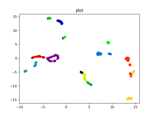
Umap Projection
Universal manifold dimensionallity reduction technique is a non linear transformation that tries to keep the distance between similar datapoints while emphasizing these one between disimilar samples. It is very useful when trying to visualize a high dimensionallity dataset where pca is discriminative enough.
Analysis Conclusion
All indexes give useful information, then the most efficient anlysis to set the clustering parameters would be to put the three of them together with some visualization tool (dimensionallity reduction).
Clustering Algorithms
Kmeans
Advantages :
- If variables are huge, then K-Means most of the times computationally faster than hierarchical clustering, if we keep k smalls.
- K-Means produce tighter clusters than hierarchical clustering, especially if the clusters are globular.
Disadvantages :
- Difficult to predict K-Value.
- With global cluster, it didn’t work well.
- Different initial partitions can result in different final clusters.
- It does not work well with different size and density clusters
Learn more: https://en.wikipedia.org/wiki/K-means_clustering
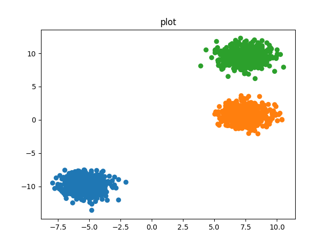
from cluster_drug_discovery.methods import kmeans
import matplotlib.pyplot as plt
cluster = kmeans.KmeansAlg(X, nclust=3)
y_pred = cluster.run()
plt.plot(X[:, 0], X[:, 1], y_pred)
Kmeans works for globular clusters:
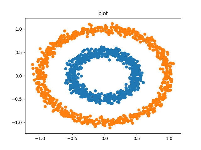
But not for density-different o converx clusters:

DBSCAN
Advantages of DBSCAN:
- Is great at separating clusters of high density versus clusters of low density within a given dataset.
- Is great with handling outliers within the dataset.
Disadvantages of DBSCAN:
- Does not work well when dealing with clusters of varying densities. While DBSCAN is great at separating high density clusters from low density clusters, DBSCAN struggles with clusters of similar density.
- Struggles with high dimensionality data. I know, this entire article I have stated how DBSCAN is great at contorting the data into different dimensions and shapes. However, DBSCAN can only go so far, if given data with too many dimensions, DBSCAN suffers
Learn more: https://en.wikipedia.org/wiki/DBSCAN
from cluster_drug_discovery.methods import dbscan
cluster = dbscan.DbscanAlg(X, nclust=3)
y_pred = cluster.run()
pl.plot(X[:, 0], X[:, 1], y_pred, output=str(i_dataset))
DBSCAN works for non globular clusters but suffers with high dimensionallity
Hierarchichal
Advantages
- No apriori information about the number of clusters required.
- Easy to implement and gives best result in some cases.
Disadvantages
- Algorithm can never undo what was done previously.
- Time complexity of at least O(n2 log n) is required, where ‘n’ is the number of data points.
- Based on the type of distance matrix chosen for merging different algorithms can suffer with outliers & complexity
Learn more: https://en.wikipedia.org/wiki/Hierarchical_clustering
from cluster_drug_discovery.methods import agglomerative
cluster = agglomerative.AgglomerativeAlg(X, nclust=3)
y_pred = cluster.run()
pl.plot(X[:, 0], X[:, 1], y_pred, output=str(i_dataset))
Agglomerative Clustering works for globular data but not convex datasets