Docking pose refinement tutorial
The aim of this tutorial is to refine a Glide docking pose of flu virus hemagglutinin inhibitor JNJ4796.
1. Protein file
We will be using a preprocessed docking pose of JNJ4796 ligand extracted from PDB 6CF7 in hemagglutinin structure (PDB code 5W6T).
You can download the structure here .
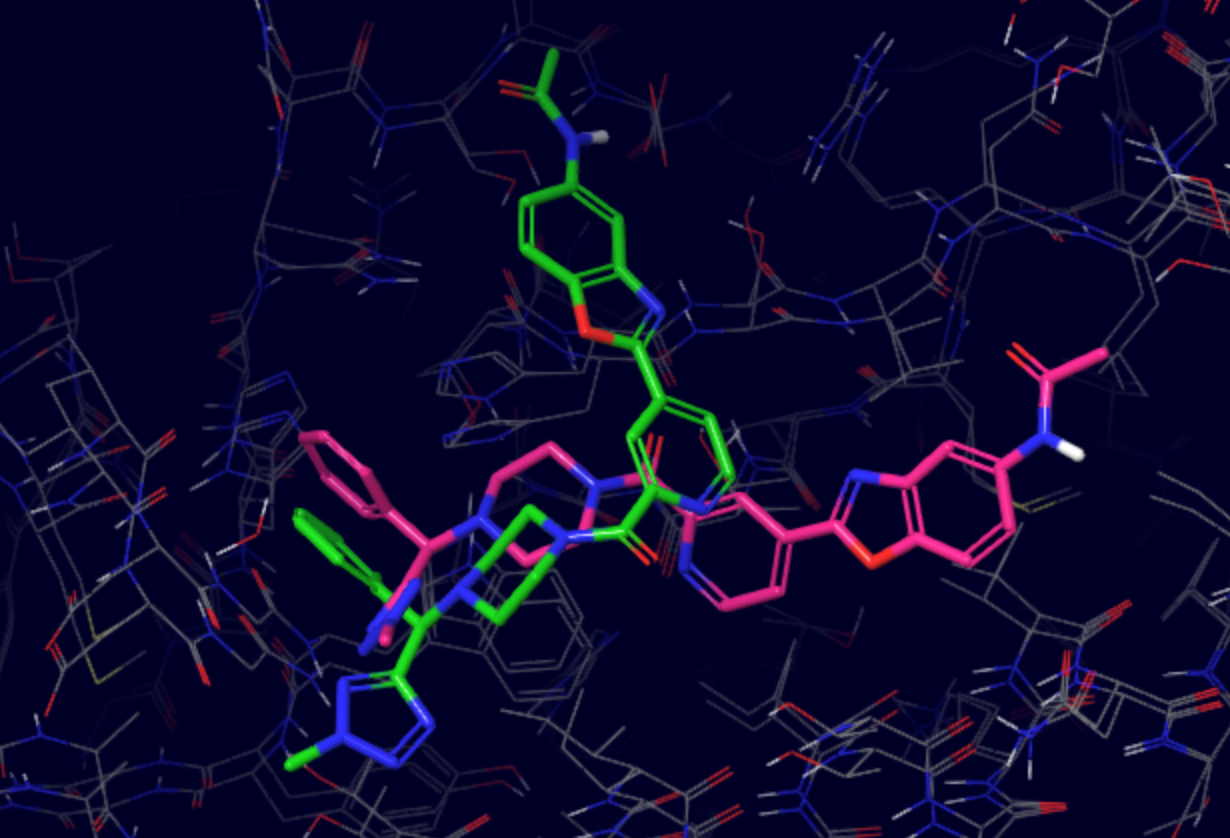
The superposition of Glide docking output (green) with the native pose (pink) resulted in the ligand RMSD of 7.68Å. Let’s see, if we can improve that with PELE’s induced fit simulation!
2. PELE input file
Create input.yaml file in your working directory, it should contain the following flags:
system - path to the protein-ligand PDB file
chain - ligand chain ID, here
Zresname - ligand residue name, in our case
LIGinduced_fit_long - to run an exhaustive induced fit simulation
atom_dist - atoms used to track the progress of the simulation, we will use one from the ligand and one from the receptor, following
chain ID:residue number:atom nameformatcpus - number of CPUs you want to use for the simulation (we suggest a minimum of 50 for a normal simulation, but you could lower it for training purposes only)
seed - random seed to ensure reproducibility.
system: 'docking.pdb'
chain: 'Z'
resname: 'LIG'
induced_fit_long: true
seed: 12345
cpus: 50
atom_dist:
- "A:29:N" # nitrogen of Ser29 in the binding site
- "Z:1:C13"
#pele_licenses: /gpfs/projects/bsc72/PELE++/mniv/V1.6.1/license/ #(Example MN4 - Need it if complain about licenses)
We strongly recommend running a test first to ensure all your input files are valid. Simply include test: true in your input.yaml and launch the simulation, it will only use 5 CPUs. If it finishes correctly, you can remove the test flag and start a full production run.
Otherwise, inspect the logs and correct any mistakes indicated in the error codes.
3. Launching the simulation
Once you have docking.pdb and input.yaml in your working directory, you can launch the simulation using one of the following methods:
directly on command line using
python -m pele_platform.main input.yamlsubmit a slurm file to the queue system (ask your IT manager, if you are not sure how to do it). In our case, the slurm file is called
slurm.sland we can launch it on the command line usingsbatch slurm.sl
Example slurm file:
#!/bin/bash
#SBATCH -J PELE
#SBATCH --output=mpi_%j.out
#SBATCH --error=mpi_%j.err
#SBATCH --ntasks=50
#SBATCH --mem-per-cpu=1000

python -m pele_platform.main input.yaml
You can download ready slurm files for MareNostrum and the NBD cluster.
If you are running the simulation on the NBD cluster, you have to include usesrun: true in your input.yaml!
4. Analysis of the results
Inside your LIG_Pele directory, you will find several folders containing simulation configuration and data, raw output as well as results folder, which
we will be mostly concerned with in this tutorial.
If you want to understand more about the content of the LIG_Pele directory, you can refer to the PELE++ documentation:
a. Plots
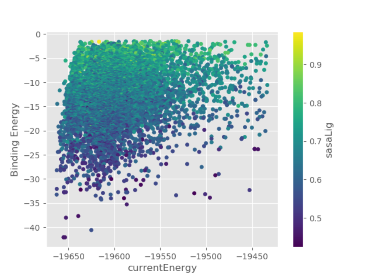
In the LIG_Pele/results/Plots folder you will find several plots, you can inspect them to get the general idea of the progression of the simulation.
For example, you can see a clear relationship between the ligand’s solvent accessible surface area and binding energy on currentEnergy_Binding_Energy_sasaLig_plot.png.
b. Selected binding modes
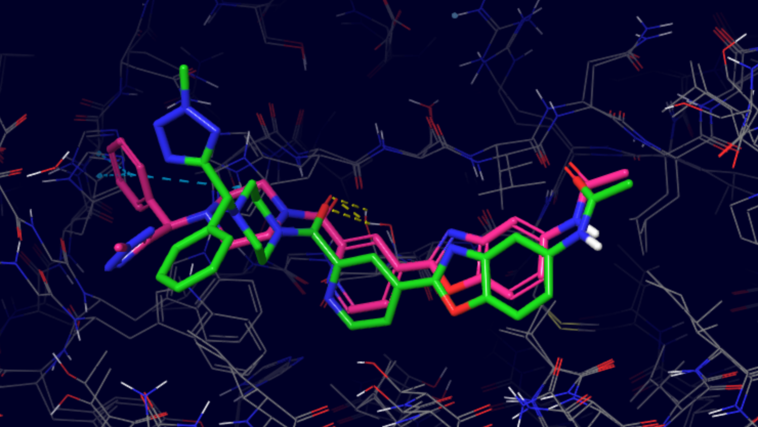
The software extracts the top 100 lowest binding energy structures in LIG_Pele/results/BestStructs/. Additionally, it clusters all poses based on
ligand heavy atom coordinates, the best energy representative of each cluster can be found in LIG_Pele/results/clusters/. The figure below shows
a representative of cluster 5 (green) superposed with the native pose (pink, PDB code 6CF7), the resulting RMSD is 4.99Å.
For more information regarding the outputs of the tutorial see Output files