Protein-protein interaction tutorial

In this tutorial we will set up a protein-protein interaction simulation aimed to elucidate a binding pocket of a bromodomain-histone inhibitor. We will be using bromodomain-containing protein 9/histone 4 X-ray structure (PDB code 4YY6) and a ligand from PDB 4UIT co-crystal.

1. Protein preparation

We will import the complex from Protein Data Bank and preprocess it using Schrödinger Maestro (release 2020-1).

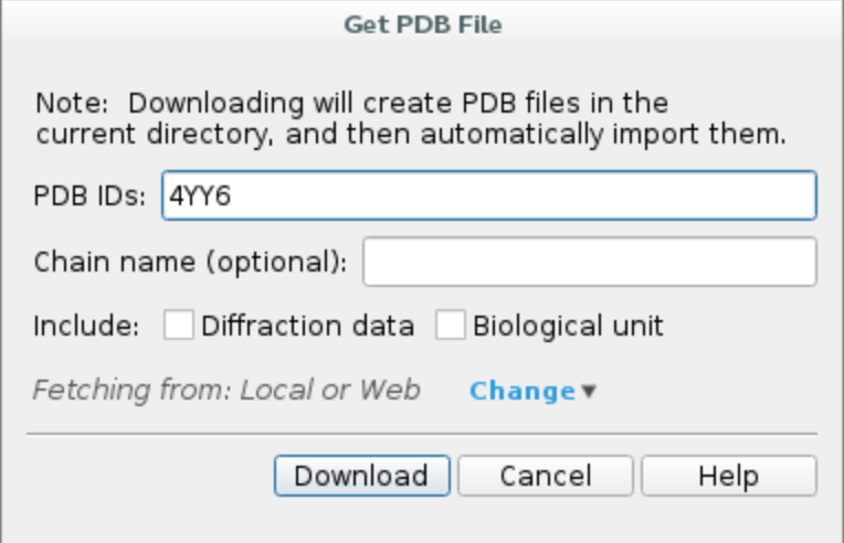
a. Launch Maestro and import the structure from PDB by clicking File -> Get PDB..., type in your PDB ID, e.g. 4YY6, and click Download. The protein structure should appear in your workspace.

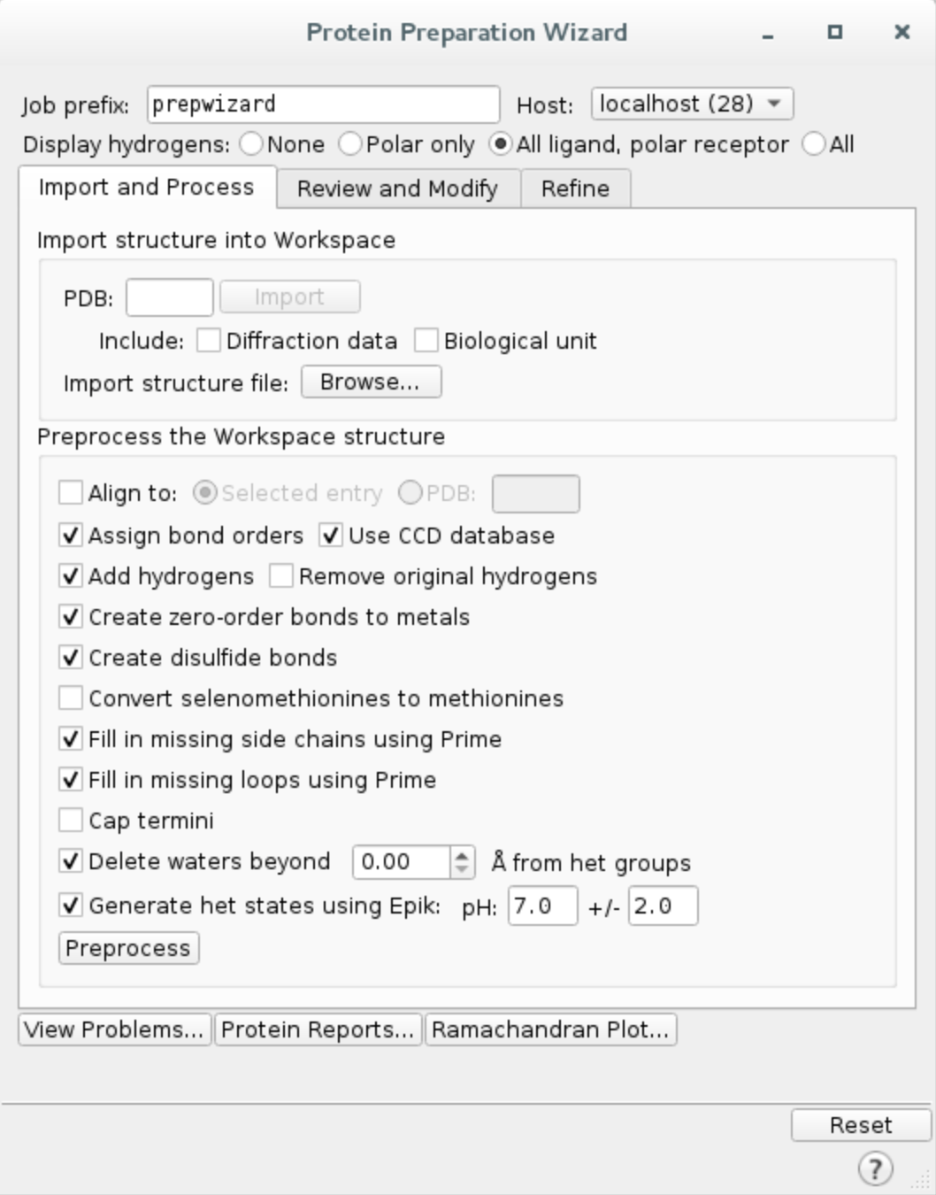
b. Preprocess the protein using Protein Preparation Wizard. Click on Tasks and search Protein Preparation Wizard. Check the following options and hit Preprocess. - Fill in missing side chain using Prime* - Fill in missing loops using Prime* - Delete waters beyond 0.0 Å from het groups (i.e. all waters in the system)

*If you do not have Prime license, you can skip those steps.

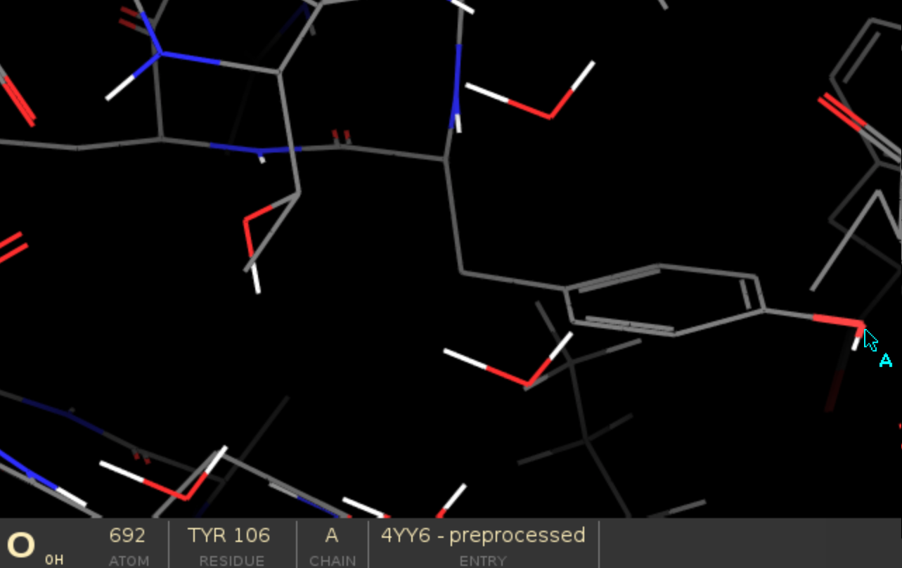
The preprocessing might take a few minutes. Upon completion, you should see 4YY6 - preprocessed on the entry list.

3. Select the centre of interface between the two proteins to guide the simulation, in this case we chose A:106:OH.

The atom strings need to follow chain ID:residue number:atom name format, you can easily check those values on the bottom panel in Maestro by hovering the mouse pointer over a specific atom.

d. Export structure by clicking on File -> Export structures... and save all workspace atoms as complex.pdb in your working directory.

2. Ligand preparation

a. Import and preprocess PDB structure 4UIT. You can ignore multiple occupancy issues, since we are only interested in the ligand.

2. Extract the ligand

   • Click on Select -> Set pick level -> Residues, then select the ligand with a mouse click

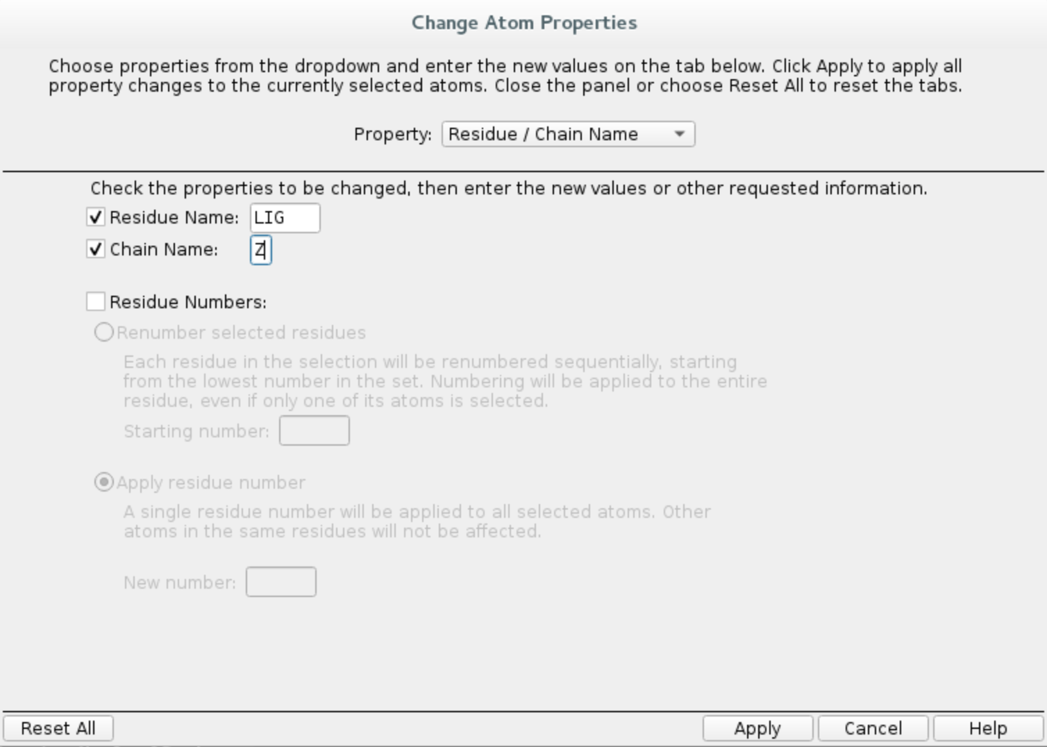
   • Open Build window and click Copy selected atoms to new entry

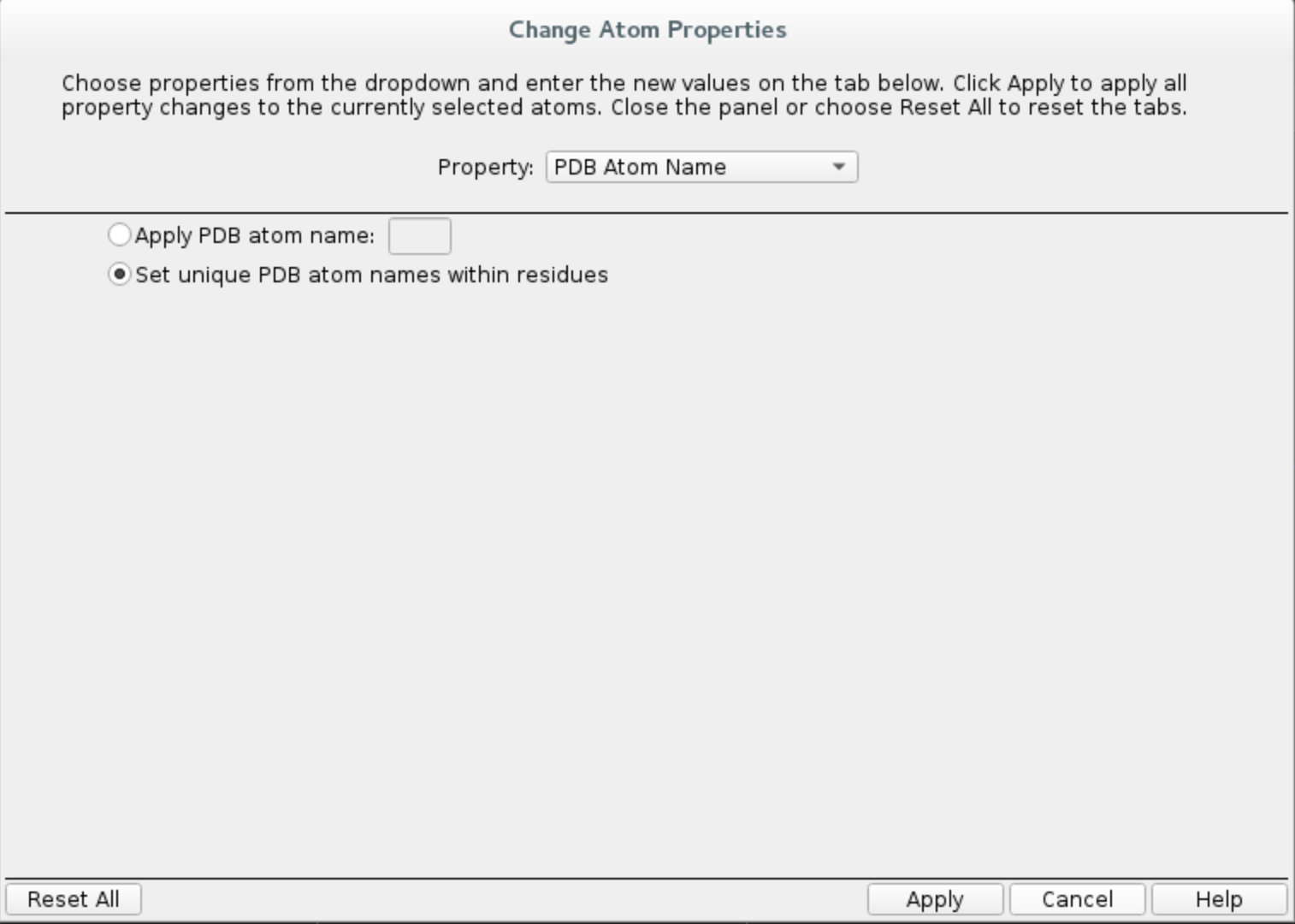
   • Select the extracted residue again and in Build window, choose Other edits -> Change atom properties...

   • Set residue name to LIG and chain name to Z

   • Choose PDB atom name from the drop down list and select Set unique PDB atom names within residues

   • Click Apply and close the window.

c. Pick atom to track progress. One of the metrics we use to follow the simulation is the distance between two selected atoms. In this case, we will pick ligand atom Z:1123:C13, then track the distance between that and the centre of interface. It will help us assess whether the ligand is forming expected interactions at the protein-protein interface or elsewhere.

d. Export the ligand by clicking on File -> Export structures... and save all workspace atoms as ligand.pdb in your working directory.

You can close Maestro now.

3. PELE input file

Create input.yaml file in your working directory, it should contain the following flags:

• system - path to the protein-protein PDB file

• ligand_pdb - PDB file with the ligand

• chain - ligand chain ID, which we set as Z in step 2b

• resname - ligand residue name, in our case LIG

• protein - chain ID of the protein chain to be kept (A, since we picked the centre of interface on A, the other chain will be automatically removed)

• center_of_interface - atom at the centre of the protein-protein interface (chain ID:residue number:atom name)

• ppi - flag to run PPI simulation

• steps - number of steps in each PELE iteration (optional)

• atom_dist - strings representing atoms selected in points 1c and 2c, used to track the progress of the simulation

• seed - random seed used in Monte Carlo steps, you should keep it consistent to ensure reproducibility of the results

• cpus - number of CPUs you want to use for the simulation (we suggest a minimum of 50 for a normal simulation, but you could lower it for training purposes only).

system: 'complex.pdb'
chain: 'Z'
protein: 'A'
ligand_pdb: "ligand.pdb"
resname: 'LIG'
center_of_interface: "A:106:OH"
seed: 12345
ppi: true
steps: 200
cpus: 50
atom_dist:
- "A:106:OH"
- "Z:1123:C13"

We strongly recommend running a test first to ensure all your input files are valid. Simply include test: true in your input.yaml and launch the simulation, it will only use 5 CPUs. If it finishes correctly, you can remove the test flag and start a full production run. Otherwise, inspect the logs and correct any mistakes indicated in the error codes.

4. Launching the simulation

Once you have complex.pdb, ligand.pdb and input.yaml in your working directory, you can launch the simulation using one of the following methods:

• directly on command line using python -m pele_platform.main input.yaml

• submit a slurm file to the queue system (ask your IT manager, if you are not sure how to do it). In our case, the slurm file is called run.sl and we can launch it on the command line using sbatch slurm.sl

Example slurm file:

#!/bin/bash
#SBATCH -J PELE
#SBATCH --output=mpi_%j.out
#SBATCH --error=mpi_%j.err
#SBATCH --ntasks=60
#SBATCH --mem-per-cpu=1000

python -m pele_platform.main input.yaml

You can download ready slurm files for MareNostrum and the NBD cluster. If you are running the simulation on the NBD cluster, you have to include usesrun: true in your input.yaml!

5. Analysis of the results

The PPI exploration consists of two steps. Initially, the position of the ligand is randomised all around the protein to perform interface exploration. Then, all results are clustered based on ligand coordinates and the best binding energy representative of each cluster is selected as input for the refinement simulation.

For the analysis part, we will only be concerned with the refinement simulation output, however, the same rules would apply to the global exploration output or any other PELE simulation.

If you want to understand more about the content of LIG_Pele directory, you can refer to the PELE++ documentation:

• Data folder

• pele.conf

• adaptive.conf

a. Plots

1. Got to LIG_Pele/2_refinement_simulation/results/Plots/ folder. It should contain a number of plots which allow you to get a general idea of the progression of the simulation.

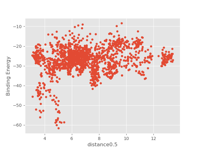
2. Examine distance0.5_Binding_Energy_plot.png showing the relationship between the binding energy and the distance between two selected atoms. Note there are few local binding energy minima, which indicates the software discovered multiple binding pockets.

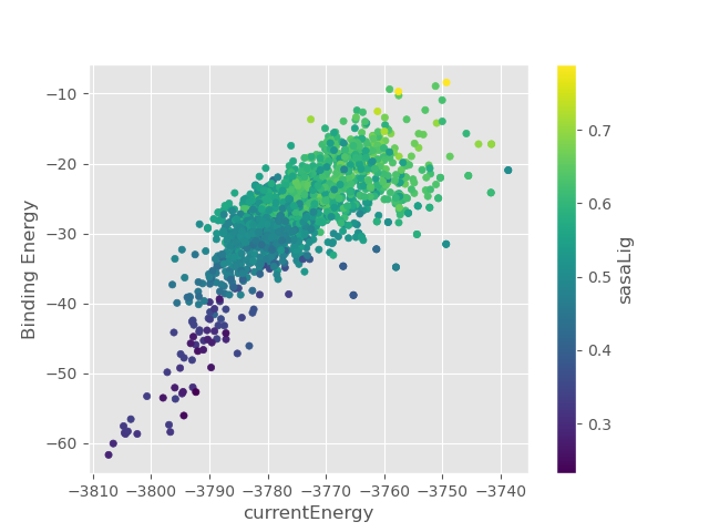
3. Take a look at currentEnergy_Binding_Energy_sasaLig_plot.png and observe how ligand’s solvent exposed surface area influences the binding energy.

Feel free to explore other plots as well.

b. Selected binding modes

1. Go to LIG_Pele/2_refinement_simulation/results folder, which contains the best binding poses split into two categories:

   • clusters contains the best binding energy representatives of each cluster

   • BestStructs holds top 100 best binding energy structures.

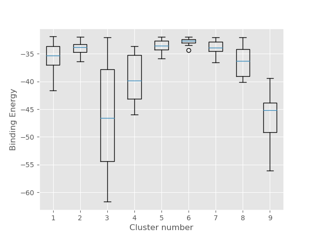
2. In the clusters folder you will find best binding energy representatives of each cluster together with a plot giving you a general overview of the binding energy distribution and median in each group. Note that most clusters have relatively high binding energies, however, cluster 3 seems to be well-populated and its representative is likely to have favourable interactions judging on the lowest energies.

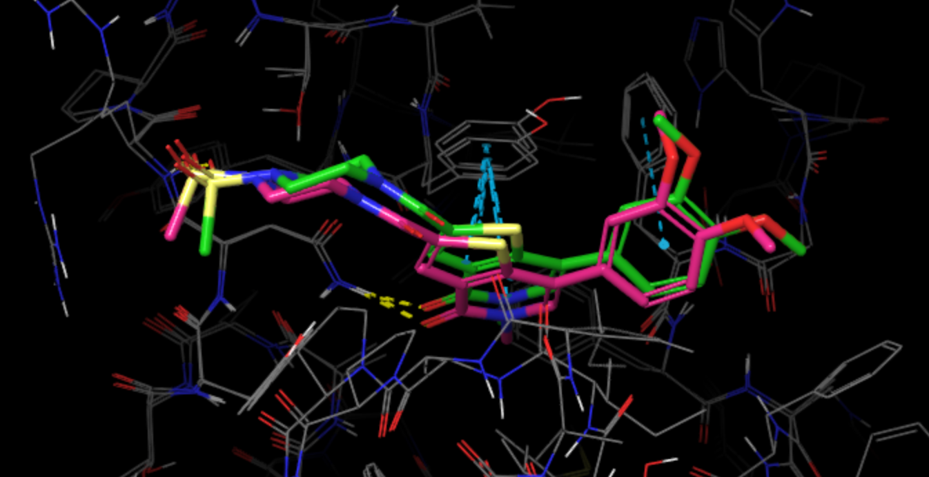
Examine cluster2_epoch0_trajectory_33.13_BindingEnergy-61.6811 structure in Maestro. Mind that PDB files are indexed starting from zero, whereas cluster numbering starts from 1, therefore cluster 2 PDB structure is, in fact, cluster 3 on the plot.

For comparison, we superposed the cluster representative structure (green) with the native pose (pink, PDB code 4UIT). The simulation was able to predict the binding pose almost perfectly, taking into account H-bonding interactions with Asn100 and Arg101 as well as pi-stacking with Tyr106.

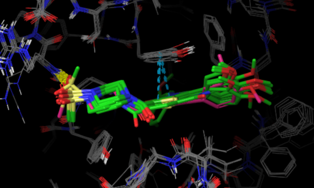
3. The BestStructs folder contains 100 PDB files with the lowest binding energy protein-ligand complexes. The picture below shows the superposition of 10 lowest energy structures (green) with the native pose (pink).

For more information regarding the outputs of the tutorial see Output files